使用 R 语言开发评分卡模型

数据准备

首先加载 scorecard 包，并载入包内自带的德国信贷数据集。该数据集包含了1000个借款人的信贷数据，20个 X 特征与1个 Y 值。其详细信息参见 UCI 的德国信贷数据集网站。

library(scorecard)

# load germancredit data
data(germancredit)

载入数据集后，可先通过变量的 IV 值、缺失率以及单类别率对 X 特征进行初步筛选。var_filter 函数默认删除信息值小于0.02、缺失率大于95%或单类别比例大于95%的变量。var_filter 函数还能够人为设定需要删除或保留的变量，以及够返回变量删除的原因列表。

# filter variable via missing rate, iv, identical rate
dt = var_filter(germancredit, y = 'creditability')

## ✔ 1 variables are removed via identical_rate
## ✔ 6 variables are removed via info_value
## ✔ Variable filtering on 1000 rows and 20 columns in 00:00:00
## ✔ 7 variables are removed in total

将经过初筛的数据集拆分为训练集与测试集。在 split_df 函数中如果指定了 y 变量，那么将基于 y 变量分层拆分，如果没有指定，则随机拆分数据集。ratio 为拆分后两个数据集的样本量占比。 seed 为随机种子，用于重现拆分的样本。

# breaking dt into train and test
dt_list = split_df(dt, y="creditability", ratio = 0.6, seed = 30)

## Warning in split_df.data.frame(dt, y = "creditability", ratio = 0.6, seed = 30):
## The ratios is set to c(0.6, 0.4)

label_list = lapply(dt_list, function(x) x$creditability)

WOE分箱

接下来对数据集进行分箱与 woe 值转换。由于这个数据集样本量比较小，我们可以直接对全样本进行分箱处理。如果数据量允许，应该使用训练集进行分箱，并使用训练集得到的 woe 值对其他数据集进行woe替换。

woebin 函数提供了树形 tree、卡方合并 chimerge、等宽 width 与等高 freq 四种分箱方法。以树形分箱为例，默认情形是当信息值增益率 stop_limit 小于0.1, 或分箱数 bin_num_limit 大于8(缺失值除外)时停止分箱，同时确保每一个分箱的样本占比 count_distr_limit 不小于5%。当然还能够通过 breaks_list 手动设定分箱节点。

woebin 函数输出的结果为多个 data.frame 组成的 list，可通过 data.table::rbindlist 或 dplyr::bind_rows 函数合并为一个数据框然后保存。当然 woebin 函数也能够直接输出一个由分箱切割点组成的 list 并保存，下次使用时直接通过 woebin 函数对 breaks_list 参数对新的数据集进行分箱。

woebin_adj 函数可逐个观察每个变量的分箱情况。如果不满意默认的分箱结果，可以手动修改。最终返回一个经过手动调整的分箱节点。

分箱之后，需要使用 woebin_ply 函数将训练集与测试集转换为对应的 woe 值。

# woe binning 
bins = woebin(dt, "creditability", print_step=0)

## ℹ Creating woe binning ...

## ✔ Binning on 1000 rows and 14 columns in 00:00:01

bins[[12]]

##                   variable           bin count count_distr neg pos   posprob
## 1: other.installment.plans bank%,%stores   186       0.186 110  76 0.4086022
## 2: other.installment.plans          none   814       0.814 590 224 0.2751843
##           woe     bin_iv   total_iv        breaks is_special_values
## 1:  0.4775508 0.04593584 0.05759207 bank%,%stores             FALSE
## 2: -0.1211786 0.01165623 0.05759207          none             FALSE

woebin_plot(bins[[12]])

## $other.installment.plans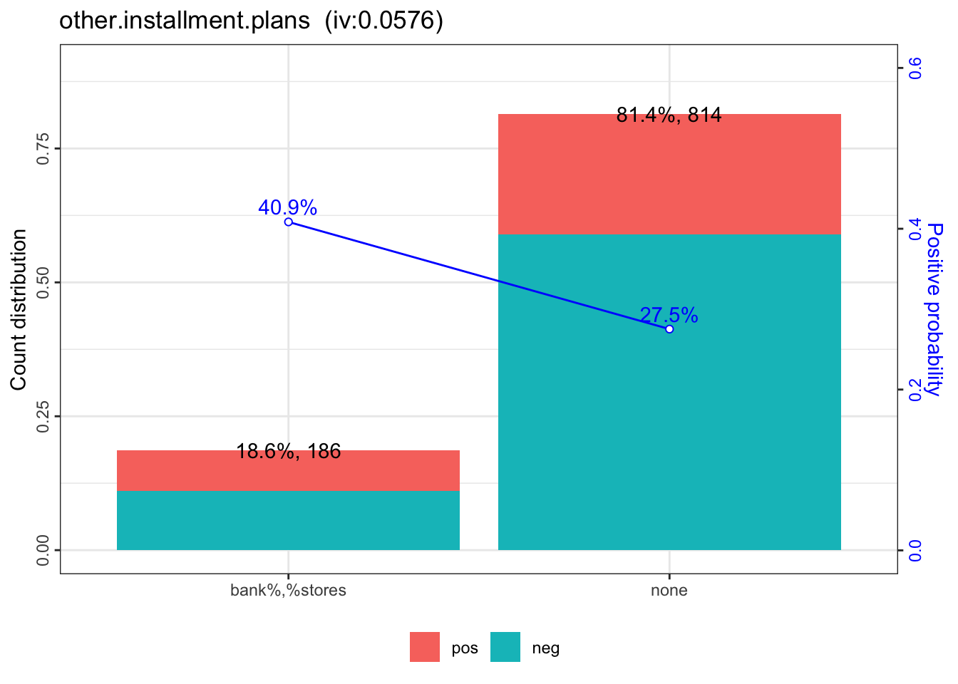

# converting train and test into woe values
dt_woe_list = lapply(dt_list, function(x) woebin_ply(x, bins))

## ℹ Converting into woe values ...

## ✔ Woe transformating on 620 rows and 13 columns in 00:00:00

## ℹ Converting into woe values ...

## ✔ Woe transformating on 380 rows and 13 columns in 00:00:00

模型拟合

当获得了 woe 值替换之后的数据集，可以使用逻辑回归进行拟合，并通过AIC、LASSO等方法对变量进一步筛选。下面使用基于 AIC 的逐步回归进一步筛选变量，最终得到了一个拥有13个变量的模型。

# lr
m1 = glm( creditability ~ ., family = binomial(), data = dt_woe_list$train)
# vif(m1, merge_coef = TRUE) # summary(m1)

# Select a formula-based model by AIC (or by LASSO for large dataset)
m_step = step(m1, direction="both", trace = FALSE)
m2 = eval(m_step$call)
vif(m2, merge_coef = TRUE) # summary(m2)

##                                                    variable   Estimate
##  1:                                             (Intercept) -0.9447617
##  2:                 status.of.existing.checking.account_woe  0.7755755
##  3:                                   duration.in.month_woe  0.7962735
##  4:                                      credit.history_woe  0.8308455
##  5:                                             purpose_woe  0.8632479
##  6:                                       credit.amount_woe  0.7669247
##  7:                           savings.account.and.bonds_woe  0.8545206
##  8: installment.rate.in.percentage.of.disposable.income_woe  1.8621446
##  9:                         other.debtors.or.guarantors_woe  2.1018289
## 10:                                        age.in.years_woe  1.0153514
## 11:                             other.installment.plans_woe  0.7622579
## 12:                                             housing_woe  0.7610232
##     Std. Error z value Pr(>|z|)     gvif
##  1:     0.1094 -8.6385   0.0000       NA
##  2:     0.1380  5.6189   0.0000 1.042054
##  3:     0.2291  3.4758   0.0005 1.180689
##  4:     0.2035  4.0823   0.0000 1.064307
##  5:     0.2755  3.1331   0.0017 1.042651
##  6:     0.2838  2.7021   0.0069 1.251179
##  7:     0.2606  3.2790   0.0010 1.038610
##  8:     0.6822  2.7296   0.0063 1.093569
##  9:     0.8922  2.3559   0.0185 1.036908
## 10:     0.3001  3.3831   0.0007 1.032968
## 11:     0.4347  1.7537   0.0795 1.059956
## 12:     0.3665  2.0767   0.0378 1.034594

模型评估

通过逻辑回归获得各变量的拟合系数之后，可以计算出各个样本为坏客户的概率，然后评估模型的预测效果。 perf_eva 函数能够计算的评估指标包括 mse, rmse, logloss, r2, ks, auc, gini，以及绘制多种可视化图形 ks, lift, gain, roc, lz, pr, f1, density。

## predicted proability
pred_list = lapply(dt_woe_list, function(x) predict(m2, x, type='response'))

## performance
perf = perf_eva(pred = pred_list, label = label_list)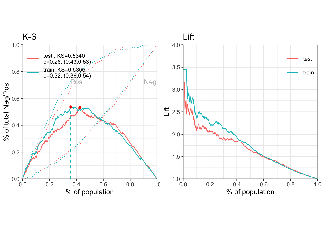

评分卡刻度

当我们获得了各个变量的分箱结果，并且确定了最终进入模型的变量以及系数，则可以创建标准评分卡。

有了评分卡之后，可用于对新样本进行打分，从而评估该客户的信用水平，并最终作出审批决策。

最后，评分卡模型的开发过程，还需要对模型的稳定性进行评估，即计算psi。

## scorecard
card = scorecard(bins, m2)
## credit score
score_list = lapply(dt_list, function(x) scorecard_ply(x, card))

## psi
perf_psi(score = score_list, label = label_list)

## $pic
## $pic$score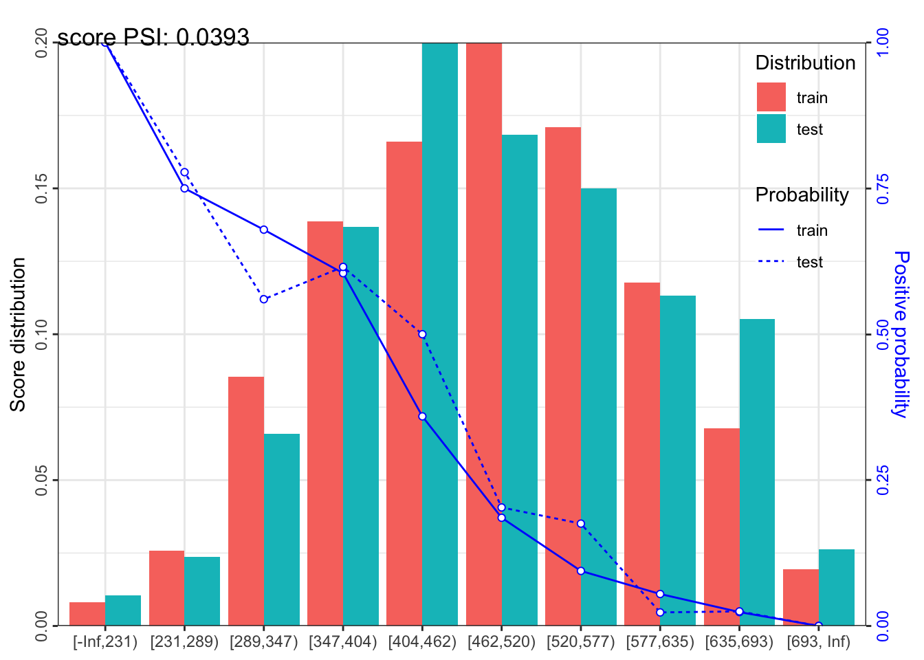

## 
## 
## $psi
##    variable    dataset        psi
## 1:    score train_test 0.03933412

以上代码均可以在该项目的主页获取。