perf_eva calculates metrics to evaluate the performance of binomial classification model. It can also creates confusion matrix and model performance graphics.
Arguments
- pred
A list or vector of predicted probability or score.
- label
A list or vector of label values.
- title
The title of plot. Defaults to NULL.
- binomial_metric
Defaults to c('mse', 'rmse', 'logloss', 'r2', 'ks', 'auc', 'gini'). If it is NULL, then no metric will calculated.
- confusion_matrix
Logical, whether to create a confusion matrix. Defaults to TRUE.
- threshold
Confusion matrix threshold. Defaults to the pred on maximum F1.
- show_plot
Defaults to c('ks', 'roc'). Accepted values including c('ks', 'lift', 'gain', 'roc', 'lz', 'pr', 'f1', 'density').
- pred_desc
whether to sort the argument of pred in descending order. Defaults to TRUE.
- positive
Value of positive class. Defaults to "bad|1".
- ...
Additional parameters.
Value
A list of binomial metric, confusion matrix and graphics
Details
Accuracy = true positive and true negative/total cases
Error rate = false positive and false negative/total cases
TPR, True Positive Rate(Recall or Sensitivity) = true positive/total actual positive
PPV, Positive Predicted Value(Precision) = true positive/total predicted positive
TNR, True Negative Rate(Specificity) = true negative/total actual negative = 1-FPR
NPV, Negative Predicted Value = true negative/total predicted negative
See also
Examples
# \donttest{
# load germancredit data
data("germancredit")
# filter variable via missing rate, iv, identical value rate
dtvf = var_filter(germancredit, "creditability")
#> ℹ Filtering variables via missing_rate, identical_rate, info_value ...
#> ✔ 1 variables are removed via identical_rate
#> ✔ 6 variables are removed via info_value
#> ✔ Variable filtering on 1000 rows and 20 columns in 00:00:00
#> ✔ 7 variables are removed in total
# breaking dt into train and test
dt_list = split_df(dtvf, "creditability")
label_list = lapply(dt_list, function(x) x$creditability)
# woe binning
bins = woebin(dt_list$train, "creditability")
#> ℹ Creating woe binning ...
#> ✔ Binning on 681 rows and 14 columns in 00:00:01
# scorecard, prob
cardprob = scorecard2(bins, dt = dt_list, y = 'creditability', return_prob = TRUE)
# credit score
score_list = lapply(dt_list, function(x) scorecard_ply(x, cardprob$card))
###### perf_eva examples ######
# Example I, one datset
## predicted p1
perf_eva(pred = cardprob$prob$train, label=label_list$train,
title = 'train')
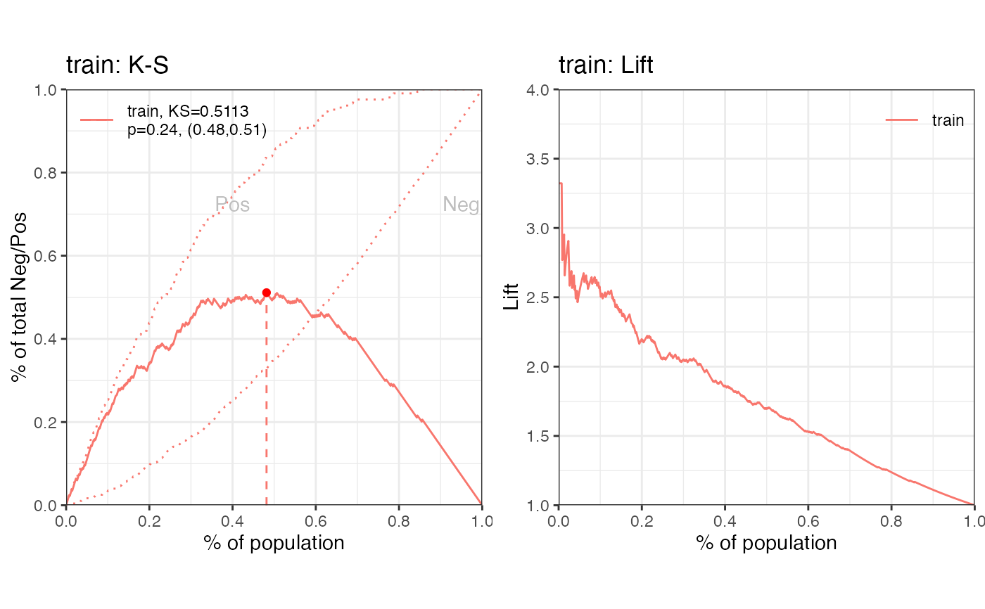 #> $binomial_metric
$train
#> MSE RMSE LogLoss R2 KS AUC Gini
#> <num> <num> <num> <num> <num> <num> <num>
#> 1: 0.1510818 0.3886924 0.4546565 0.2819652 0.5112933 0.8308414 0.6616827
#>
#>
#> $pic
#> TableGrob (1 x 2) "arrange": 2 grobs
#> z cells name grob
#> 1 1 (1-1,1-1) arrange gtable[layout]
#> 2 2 (1-1,2-2) arrange gtable[layout]
#>
## predicted score
# perf_eva(pred = score_list$train, label=label_list$train,
# title = 'train')
# Example II, multiple datsets
## predicted p1
perf_eva(pred = cardprob$prob, label = label_list,
show_plot = c('ks', 'lift', 'gain', 'roc', 'lz', 'pr', 'f1', 'density'))
#> $binomial_metric
#> $binomial_metric$train
#> MSE RMSE LogLoss R2 KS AUC Gini
#> <num> <num> <num> <num> <num> <num> <num>
#> 1: 0.1510818 0.3886924 0.4546565 0.2819652 0.5112933 0.8308414 0.6616827
#>
#>
#> $pic
#> TableGrob (1 x 2) "arrange": 2 grobs
#> z cells name grob
#> 1 1 (1-1,1-1) arrange gtable[layout]
#> 2 2 (1-1,2-2) arrange gtable[layout]
#>
## predicted score
# perf_eva(pred = score_list$train, label=label_list$train,
# title = 'train')
# Example II, multiple datsets
## predicted p1
perf_eva(pred = cardprob$prob, label = label_list,
show_plot = c('ks', 'lift', 'gain', 'roc', 'lz', 'pr', 'f1', 'density'))
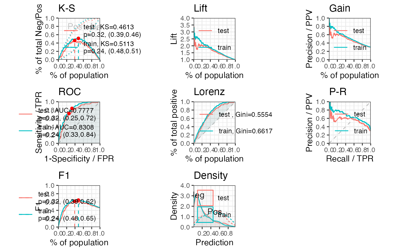 #> $binomial_metric
$train
#> MSE RMSE LogLoss R2 KS AUC Gini
#> <num> <num> <num> <num> <num> <num> <num>
#> 1: 0.1510818 0.3886924 0.4546565 0.2819652 0.5112933 0.8308414 0.6616827
#>
#> $binomial_metric$test
#> MSE RMSE LogLoss R2 KS AUC Gini
#> <num> <num> <num> <num> <num> <num> <num>
#> 1: 0.1697538 0.4120119 0.5118995 0.1882372 0.4613252 0.7777021 0.5554041
#>
#>
#> $pic
#> TableGrob (3 x 3) "arrange": 8 grobs
#> z cells name grob
#> 1 1 (1-1,1-1) arrange gtable[layout]
#> 2 2 (1-1,2-2) arrange gtable[layout]
#> 3 3 (1-1,3-3) arrange gtable[layout]
#> 4 4 (2-2,1-1) arrange gtable[layout]
#> 5 5 (2-2,2-2) arrange gtable[layout]
#> 6 6 (2-2,3-3) arrange gtable[layout]
#> 7 7 (3-3,1-1) arrange gtable[layout]
#> 8 8 (3-3,2-2) arrange gtable[layout]
#>
## predicted score
# perf_eva(score_list, label_list)
# }
#> $binomial_metric
#> $binomial_metric$train
#> MSE RMSE LogLoss R2 KS AUC Gini
#> <num> <num> <num> <num> <num> <num> <num>
#> 1: 0.1510818 0.3886924 0.4546565 0.2819652 0.5112933 0.8308414 0.6616827
#>
#> $binomial_metric$test
#> MSE RMSE LogLoss R2 KS AUC Gini
#> <num> <num> <num> <num> <num> <num> <num>
#> 1: 0.1697538 0.4120119 0.5118995 0.1882372 0.4613252 0.7777021 0.5554041
#>
#>
#> $pic
#> TableGrob (3 x 3) "arrange": 8 grobs
#> z cells name grob
#> 1 1 (1-1,1-1) arrange gtable[layout]
#> 2 2 (1-1,2-2) arrange gtable[layout]
#> 3 3 (1-1,3-3) arrange gtable[layout]
#> 4 4 (2-2,1-1) arrange gtable[layout]
#> 5 5 (2-2,2-2) arrange gtable[layout]
#> 6 6 (2-2,3-3) arrange gtable[layout]
#> 7 7 (3-3,1-1) arrange gtable[layout]
#> 8 8 (3-3,2-2) arrange gtable[layout]
#>
## predicted score
# perf_eva(score_list, label_list)
# }